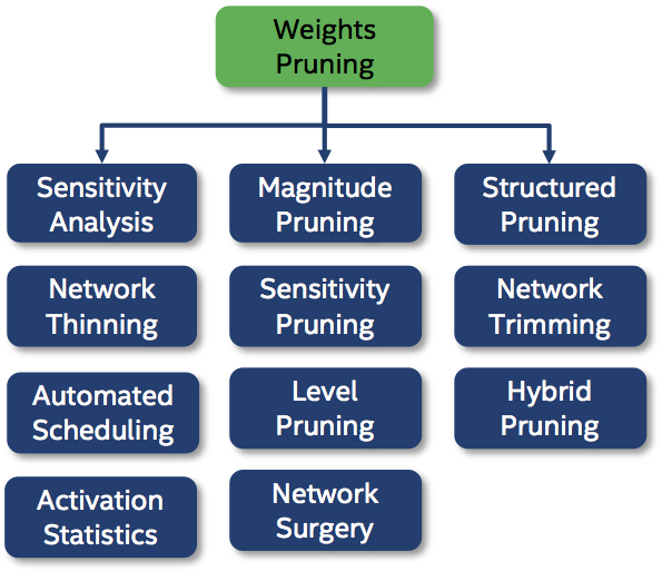
Weights Pruning Algorithms

Magnitude Pruner

This is the most basic pruner: it applies a thresholding function, \(thresh(.)\), on each element, \(w_i\), of a weights tensor. A different threshold can be used for each layer's weights tensor.
Because the threshold is applied on individual elements, this pruner belongs to the element-wise pruning algorithm family.

\[ thresh(w_i)=\left\lbrace \matrix{{{w_i: \; if \;|w_i| \; \gt}\;\lambda}\cr {0: \; if \; |w_i| \leq \lambda} } \right\rbrace \]

Sensitivity Pruner

Finding a threshold magnitude per layer is daunting, especially since each layer's elements have different average absolute values. We can take advantage of the fact that the weights of convolutional and fully connected layers exhibit a Gaussian distribution with a mean value roughly zero, to avoid using a direct threshold based on the values of each specific tensor.
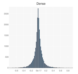
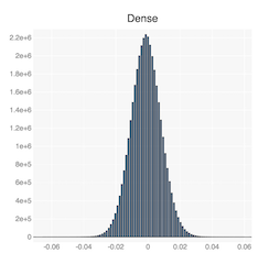
The diagram below shows the distribution the weights tensor of the first convolutional layer, and first fully-connected layer in TorchVision's pre-trained Alexnet model. You can see that they have an approximate Gaussian distribution.

The distributions of Alexnet conv1 and fc1 layers

We use the standard deviation of the weights tensor as a sort of normalizing factor between the different weights tensors. For example, if a tensor is Normally distributed, then about 68% of the elements have an absolute value less than the standard deviation (\(\sigma\)) of the tensor. Thus, if we set the threshold to \(s*\sigma\), then basically we are thresholding \(s * 68\%\) of the tensor elements.

\[ thresh(w_i)=\left\lbrace \matrix{{{w_i: \; if \;|w_i| \; \gt}\;\lambda}\cr {0: \; if \; |w_i| \leq \lambda} } \right\rbrace \]

\[ \lambda = s * \sigma_l \;\;\; where\; \sigma_l\; is \;the \;std \;of \;layer \;l \;as \;measured \;on \;the \;dense \;model \]

How do we choose this \(s\) multiplier?

In Learning both Weights and Connections for Efficient Neural Networks the authors write:

"We used the sensitivity results to find each layer’s threshold: for example, the smallest threshold was applied to the most sensitive layer, which is the first convolutional layer... The pruning threshold is chosen as a quality parameter multiplied by the standard deviation of a layer’s weights

So the results of executing pruning sensitivity analysis on the tensor, gives us a good starting guess at \(s\). Sensitivity analysis is an empirical method, and we still have to spend time to hone in on the exact multiplier value.

Method of Operation

Start by running a pruning sensitivity analysis on the model.
Then use the results to set and tune the threshold of each layer, but instead of using a direct threshold use a sensitivity parameter which is multiplied by the standard-deviation of the initial weight-tensor's distribution.

Schedule

In their paper Song Han et al. use iterative pruning and change the value of the \(s\) multiplier at each pruning step. Distiller's SensitivityPruner works differently: the value \(s\) is set once based on a one-time calculation of the standard-deviation of the tensor (the first time we prune), and relies on the fact that as the tensor is pruned, more elements are "pulled" toward the center of the distribution and thus more elements gets pruned.

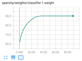
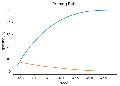
This actually works quite well as we can see in the diagram below. This is a TensorBoard screen-capture from Alexnet training, which shows how this method starts off pruning very aggressively, but then slowly reduces the pruning rate.

We use a simple iterative-pruning schedule such as: Prune every second epoch starting at epoch 0, and ending at epoch 38. This excerpt from alexnet.schedule_sensitivity.yaml shows how this iterative schedule is conveyed in Distiller scheduling configuration YAML:

pruners:
  my_pruner:
    class: 'SensitivityPruner'
    sensitivities:
      'features.module.0.weight': 0.25
      'features.module.3.weight': 0.35
      'features.module.6.weight': 0.40
      'features.module.8.weight': 0.45
      'features.module.10.weight': 0.55
      'classifier.1.weight': 0.875
      'classifier.4.weight': 0.875
      'classifier.6.weight': 0.625

policies:
  - pruner:
      instance_name : 'my_pruner'
    starting_epoch: 0
    ending_epoch: 38
    frequency: 2

Level Pruner

Class SparsityLevelParameterPruner uses a similar method to go around specifying specific thresholding magnitudes. Instead of specifying a threshold magnitude, you specify a target sparsity level (expressed as a fraction, so 0.5 means 50% sparsity). Essentially this pruner also uses a pruning criteria based on the magnitude of each tensor element, but it has the advantage that you can aim for an exact and specific sparsity level.

This pruner is much more stable compared to SensitivityPruner because the target sparsity level is not coupled to the actual magnitudes of the elements. Distiller's SensitivityPruner is unstable because the final sparsity level depends on the convergence pattern of the tensor distribution. Song Han's methodology of using several different values for the multiplier \(s\), and the recalculation of the standard-deviation at each pruning phase, probably gives it stability, but requires much more hyper-parameters (this is the reason we have not implemented it thus far).

To set the target sparsity levels, you can once again use pruning sensitivity analysis to make better guesses at the correct sparsity level of each

Method of Operation

Sort the weights in the specified layer by their absolute values.
Mask to zero the smallest magnitude weights until the desired sparsity level is reached.

Splicing Pruner

In Dynamic Network Surgery for Efficient DNNs Guo et. al propose that network pruning and splicing work in tandem. A SpilicingPruner is a pruner that both prunes and splices connections and works best with a Dynamic Network Surgery schedule, which, for example, configures the PruningPolicy to mask weights only during the forward pass.

Automated Gradual Pruner (AGP)

In To prune, or not to prune: exploring the efficacy of pruning for model compression, authors Michael Zhu and Suyog Gupta provide an algorithm to schedule a Level Pruner which Distiller implements in AutomatedGradualPruner.

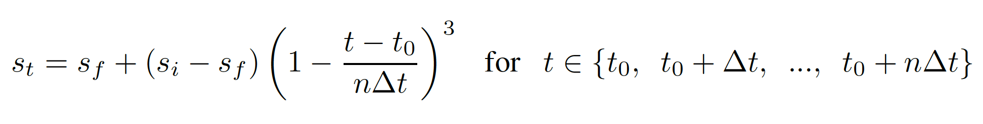
"We introduce a new automated gradual pruning algorithm in which the sparsity is increased from an initial sparsity value \(s_i\) (usually 0) to a ﬁnal sparsity value \(s_f\) over a span of n pruning steps. The intuition behind this sparsity function in equation (1) is to prune the network rapidly in the initial phase when the redundant connections are abundant and gradually reduce the number of weights being pruned each time as there are fewer and fewer weights remaining in the network.""

You can play with the scheduling parameters in the agp_schedule.ipynb notebook.

The authors describe AGP:

Our automated gradual pruning algorithm prunes the smallest magnitude weights to achieve a preset level of network sparsity.

Doesn't require much hyper-parameter tuning

Shown to perform well across different models

Does not make any assumptions about the structure of the network or its constituent layers, and is therefore more generally applicable.

RNN Pruner

The authors of Exploring Sparsity in Recurrent Neural Networks, Sharan Narang, Erich Elsen, Gregory Diamos, and Shubho Sengupta, "propose a technique to reduce the parameters of a network by pruning weights during the initial training of the network." They use a gradual pruning schedule which is reminiscent of the schedule used in AGP, for element-wise pruning of RNNs, which they also employ during training. They show pruning of RNN, GRU, LSTM and embedding layers.

Distiller's distiller.pruning.BaiduRNNPruner class implements this pruning algorithm.

Structure Pruners

Element-wise pruning can create very sparse models which can be compressed to consume less memory footprint and bandwidth, but without specialized hardware that can compute using the sparse representation of the tensors, we don't gain any speedup of the computation. Structure pruners, remove entire "structures", such as kernels, filters, and even entire feature-maps.

Structure Ranking Pruners

Ranking pruners use some criterion to rank the structures in a tensor, and then prune the tensor to a specified level. In principle, these pruners perform one-shot pruning, but can be combined with automatic pruning-level scheduling, such as AGP (see below). In Pruning Filters for Efficient ConvNets the authors use filter ranking, with one-shot pruning followed by fine-tuning. The authors of Exploiting Sparseness in Deep Neural Networks for Large Vocabulary Speech Recognition also use a one-shot pruning schedule, for fully-connected layers, and they provide an explanation:

First, after sweeping through the full training set several times the weights become relatively stable — they tend to remain either large or small magnitudes. Second, in a stabilized model, the importance of the connection is approximated well by the magnitudes of the weights (times the magnitudes of the corresponding input values, but these are relatively uniform within each layer since on the input layer, features are normalized to zero-mean and unit-variance, and hidden-layer values are probabilities)

L1RankedStructureParameterPruner

The L1RankedStructureParameterPruner pruner calculates the magnitude of some "structure", orders all of the structures based on some magnitude function and the m lowest ranking structures are pruned away. This pruner performs ranking of structures using the mean of the absolute value of the structure as the representative of the structure magnitude. The absolute mean does not depend on the size of the structure, so it is easier to use compared to just using the \(L_1\)-norm of the structure, and at the same time it is a good proxy of the \(L_1\)-norm. Basically, you can think of mean(abs(t)) as a form of normalization of the structure L1-norm by the length of the structure. L1RankedStructureParameterPruner currently prunes weight filters, channels, and rows (for linear layers).

ActivationAPoZRankedFilterPruner

The ActivationAPoZRankedFilterPruner pruner uses the activation channels mean APoZ (average percentage of zeros) to rank weight filters and prune a specified percentage of filters. This method is called Network Trimming from the research paper: "Network Trimming: A Data-Driven Neuron Pruning Approach towards Efficient Deep Architectures", Hengyuan Hu, Rui Peng, Yu-Wing Tai, Chi-Keung Tang, ICLR 2016 https://arxiv.org/abs/1607.03250

GradientRankedFilterPruner

The GradientRankedFilterPruner tries to asses the importance of weight filters using the product of their gradients and the filter value.

RandomRankedFilterPruner

For research purposes we may want to compare the results of some structure-ranking pruner to a random structure-ranking. The RandomRankedFilterPruner pruner can be used for this purpose.

Automated Gradual Pruner (AGP) for Structures

The idea of a mathematical formula controlling the sparsity level growth is very useful and StructuredAGP extends the implementation to structured pruning.

Pruner Compositions

Pruners can be combined to create new pruning schemes. Specifically, with a few lines of code we currently marry the AGP sparsity level scheduler with our filter-ranking classes to create pruner compositions. For each of these, we use AGP to decided how many filters to prune at each step, and we choose the filters to remove using one of the filter-ranking methods:

L1RankedStructureParameterPruner_AGP
ActivationAPoZRankedFilterPruner_AGP
GradientRankedFilterPruner_AGP
RandomRankedFilterPruner_AGP

Hybrid Pruning

In a single schedule we can mix different pruning techniques. For example, we might mix pruning and regularization. Or structured pruning and element-wise pruning. We can even apply different methods on the same tensor. For example, we might want to perform filter pruning for a few epochs, then perform thinning and continue with element-wise pruning of the smaller network tensors. This technique of mixing different methods we call Hybrid Pruning, and Distiller has a few example schedules.