Distiller Model Zoo
Note: Checkpoint files are no longer provided. We're still keeping this page for those who may find the discussions useful.
Contents
The Distiller model zoo is not a "traditional" model-zoo, because it does not necessarily contain best-in-class compressed models. Instead, the model-zoo contains a number of deep learning models that have been compressed using Distiller following some well-known research papers. These are meant to serve as examples of how Distiller can be used.
Each model contains a Distiller schedule detailing how the model was compressed, a PyTorch checkpoint, text logs and TensorBoard logs.
| Paper | Dataset | Network | Method & Granularity | Schedule | Features |
|---|---|---|---|---|---|
| Learning both Weights and Connections for Efficient Neural Networks | ImageNet | Alexnet | Element-wise pruning | Iterative; Manual | Magnitude thresholding based on a sensitivity quantifier. Element-wise sparsity sensitivity analysis |
| To prune, or not to prune: exploring the efficacy of pruning for model compression | ImageNet | MobileNet | Element-wise pruning | Automated gradual; Iterative | Magnitude thresholding based on target level |
| Learning Structured Sparsity in Deep Neural Networks | CIFAR10 | ResNet20 | Group regularization | 1.Train with group-lasso 2.Remove zero groups and fine-tune |
Group Lasso regularization. Groups: kernels (2D), channels, filters (3D), layers (4D), vectors (rows, cols) |
| Pruning Filters for Efficient ConvNets | CIFAR10 | ResNet56 | Filter ranking; guided by sensitivity analysis | 1.Rank filters 2. Remove filters and channels 3.Fine-tune |
One-shot ranking and pruning of filters; with network thinning |
Learning both Weights and Connections for Efficient Neural Networks
This schedule is an example of "Iterative Pruning" for Alexnet/Imagent, as described in chapter 3 of Song Han's PhD dissertation: Efficient Methods and Hardware for Deep Learning and in his paper Learning both Weights and Connections for Efficient Neural Networks.
The Distiller schedule uses SensitivityPruner which is similar to MagnitudeParameterPruner, but instead of specifying "raw" thresholds, it uses a "sensitivity parameter". Song Han's paper says that "the pruning threshold is chosen as a quality parameter multiplied by the standard deviation of a layers weights," and this is not explained much further. In Distiller, the "quality parameter" is referred to as "sensitivity" and is based on the values learned from performing sensitivity analysis. Using a parameter that is related to the standard deviation is very helpful: under the assumption that the weights tensors are distributed normally, the standard deviation acts as a threshold normalizer.
Note that Distiller's implementation deviates slightly from the algorithm Song Han describes in his PhD dissertation, in that the threshold value is set only once. In his PhD dissertation, Song Han describes a growing threshold, at each iteration. This requires n+1 hyper-parameters (n being the number of pruning iterations we use): the threshold and the threshold increase (delta) at each pruning iteration. Distiller's implementation takes advantage of the fact that as pruning progresses, more weights are pulled toward zero, and therefore the threshold "traps" more weights. Thus, we can use less hyper-parameters and achieve the same results.
- Distiller schedule:
distiller/examples/sensitivity-pruning/alexnet.schedule_sensitivity.yaml
Results
Our reference is TorchVision's pretrained Alexnet model which has a Top1 accuracy of 56.55 and Top5=79.09. We prune away 88.44% of the parameters and achieve Top1=56.61 and Top5=79.45. Song Han prunes 89% of the parameters, which is slightly better than our results.
Parameters:
+----+---------------------------+------------------+---------------+----------------+------------+------------+----------+----------+----------+------------+---------+----------+------------+
|    | Name                      | Shape            |   NNZ (dense) |   NNZ (sparse) |   Cols (%) |   Rows (%) |   Ch (%) |   2D (%) |   3D (%) |   Fine (%) |     Std |     Mean |   Abs-Mean
|----+---------------------------+------------------+---------------+----------------+------------+------------+----------+----------+----------+------------+---------+----------+------------|
|  0 | features.module.0.weight  | (64, 3, 11, 11)  |         23232 |          13411 |    0.00000 |    0.00000 |  0.00000 |  0.00000 |  0.00000 |   42.27359 | 0.14391 | -0.00002 |    0.08805 |
|  1 | features.module.3.weight  | (192, 64, 5, 5)  |        307200 |         115560 |    0.00000 |    0.00000 |  0.00000 |  1.91243 |  0.00000 |   62.38281 | 0.04703 | -0.00250 |    0.02289 |
|  2 | features.module.6.weight  | (384, 192, 3, 3) |        663552 |         256565 |    0.00000 |    0.00000 |  0.00000 |  6.18490 |  0.00000 |   61.33445 | 0.03354 | -0.00184 |    0.01803 |
|  3 | features.module.8.weight  | (256, 384, 3, 3) |        884736 |         315065 |    0.00000 |    0.00000 |  0.00000 |  6.96411 |  0.00000 |   64.38881 | 0.02646 | -0.00168 |    0.01422 |
|  4 | features.module.10.weight | (256, 256, 3, 3) |        589824 |         186938 |    0.00000 |    0.00000 |  0.00000 | 15.49225 |  0.00000 |   68.30614 | 0.02714 | -0.00246 |    0.01409 |
|  5 | classifier.1.weight       | (4096, 9216)     |      37748736 |        3398881 |    0.00000 |    0.21973 |  0.00000 |  0.21973 |  0.00000 |   90.99604 | 0.00589 | -0.00020 |    0.00168 |
|  6 | classifier.4.weight       | (4096, 4096)     |      16777216 |        1782769 |    0.21973 |    3.46680 |  0.00000 |  3.46680 |  0.00000 |   89.37387 | 0.00849 | -0.00066 |    0.00263 |
|  7 | classifier.6.weight       | (1000, 4096)     |       4096000 |         994738 |    3.36914 |    0.00000 |  0.00000 |  0.00000 |  0.00000 |   75.71440 | 0.01718 |  0.00030 |    0.00778 |
|  8 | Total sparsity:           | -                |      61090496 |        7063928 |    0.00000 |    0.00000 |  0.00000 |  0.00000 |  0.00000 |   88.43694 | 0.00000 |  0.00000 |    0.00000 |
+----+---------------------------+------------------+---------------+----------------+------------+------------+----------+----------+----------+------------+---------+----------+------------+
 2018-04-04 21:30:52,499 - Total sparsity: 88.44

 2018-04-04 21:30:52,499 - --- validate (epoch=89)-----------
 2018-04-04 21:30:52,499 - 128116 samples (256 per mini-batch)
 2018-04-04 21:31:35,357 - ==> Top1: 51.838    Top5: 74.817    Loss: 2.150

 2018-04-04 21:31:39,251 - --- test ---------------------
 2018-04-04 21:31:39,252 - 50000 samples (256 per mini-batch)
 2018-04-04 21:32:01,274 - ==> Top1: 56.606    Top5: 79.446    Loss: 1.893
To prune, or not to prune: exploring the efficacy of pruning for model compression
In their paper Zhu and Gupta, "compare the accuracy of large, but pruned models (large-sparse) and their smaller, but dense (small-dense) counterparts with identical memory footprint." They also "propose a new gradual pruning technique that is simple and straightforward to apply across a variety of models/datasets with minimal tuning."
This pruning schedule is implemented by distiller.AutomatedGradualPruner, which increases the sparsity level (expressed as a percentage of zero-valued elements) gradually over several pruning steps. Distiller's implementation only prunes elements once in an epoch (the model is fine-tuned in between pruning events), which is a small deviation from Zhu and Gupta's paper. The research paper specifies the schedule in terms of mini-batches, while our implementation specifies the schedule in terms of epochs. We feel that using epochs performs well, and is more "stable", since the number of mini-batches will change, if you change the batch size.
ImageNet files:
- Distiller schedule:
distiller/examples/agp-pruning/mobilenet.imagenet.schedule_agp.yaml
ResNet18 files:
- Distiller schedule:
distiller/examples/agp-pruning/resnet18.schedule_agp.yaml
Results
As our baseline we used a pretrained PyTorch MobileNet model (width=1) which has Top1=68.848 and Top5=88.740.
In their paper, Zhu and Gupta prune 50% of the elements of MobileNet (width=1) with a 1.1% drop in accuracy. We pruned about 51.6% of the elements, with virtually no change in the accuracies (Top1: 68.808 and Top5: 88.656). We didn't try to prune more than this, but we do note that the baseline accuracy that we used is almost 2% lower than the accuracy published in the paper.
+----+--------------------------+--------------------+---------------+----------------+------------+------------+----------+----------+----------+------------+---------+----------+------------+
|    | Name                     | Shape              |   NNZ (dense) |   NNZ (sparse) |   Cols (%) |   Rows (%) |   Ch (%) |   2D (%) |   3D (%) |   Fine (%) |     Std |     Mean |   Abs-Mean |
|----+--------------------------+--------------------+---------------+----------------+------------+------------+----------+----------+----------+------------+---------+----------+------------|
|  0 | module.model.0.0.weight  | (32, 3, 3, 3)      |           864 |            864 |    0.00000 |    0.00000 |  0.00000 |  0.00000 |  0.00000 |    0.00000 | 0.14466 |  0.00103 |    0.06508 |
|  1 | module.model.1.0.weight  | (32, 1, 3, 3)      |           288 |            288 |    0.00000 |    0.00000 |  0.00000 |  0.00000 |  0.00000 |    0.00000 | 0.32146 |  0.01020 |    0.12932 |
|  2 | module.model.1.3.weight  | (64, 32, 1, 1)     |          2048 |           2048 |    0.00000 |    0.00000 |  0.00000 |  0.00000 |  0.00000 |    0.00000 | 0.11942 |  0.00024 |    0.03627 |
|  3 | module.model.2.0.weight  | (64, 1, 3, 3)      |           576 |            576 |    0.00000 |    0.00000 |  0.00000 |  0.00000 |  0.00000 |    0.00000 | 0.15809 |  0.00543 |    0.11513 |
|  4 | module.model.2.3.weight  | (128, 64, 1, 1)    |          8192 |           8192 |    0.00000 |    0.00000 |  0.00000 |  0.00000 |  0.00000 |    0.00000 | 0.08442 | -0.00031 |    0.04182 |
|  5 | module.model.3.0.weight  | (128, 1, 3, 3)     |          1152 |           1152 |    0.00000 |    0.00000 |  0.00000 |  0.00000 |  0.00000 |    0.00000 | 0.16780 |  0.00125 |    0.10545 |
|  6 | module.model.3.3.weight  | (128, 128, 1, 1)   |         16384 |          16384 |    0.00000 |    0.00000 |  0.00000 |  0.00000 |  0.00000 |    0.00000 | 0.07126 | -0.00197 |    0.04123 |
|  7 | module.model.4.0.weight  | (128, 1, 3, 3)     |          1152 |           1152 |    0.00000 |    0.00000 |  0.00000 |  0.00000 |  0.00000 |    0.00000 | 0.10182 |  0.00171 |    0.08719 |
|  8 | module.model.4.3.weight  | (256, 128, 1, 1)   |         32768 |          13108 |    0.00000 |    0.00000 | 10.15625 | 59.99756 | 12.50000 |   59.99756 | 0.05543 | -0.00002 |    0.02760 |
|  9 | module.model.5.0.weight  | (256, 1, 3, 3)     |          2304 |           2304 |    0.00000 |    0.00000 |  0.00000 |  0.00000 |  0.00000 |    0.00000 | 0.12516 | -0.00288 |    0.08058 |
| 10 | module.model.5.3.weight  | (256, 256, 1, 1)   |         65536 |          26215 |    0.00000 |    0.00000 | 12.50000 | 59.99908 | 23.82812 |   59.99908 | 0.04453 |  0.00002 |    0.02271 |
| 11 | module.model.6.0.weight  | (256, 1, 3, 3)     |          2304 |           2304 |    0.00000 |    0.00000 |  0.00000 |  0.00000 |  0.00000 |    0.00000 | 0.08024 |  0.00252 |    0.06377 |
| 12 | module.model.6.3.weight  | (512, 256, 1, 1)   |        131072 |          52429 |    0.00000 |    0.00000 | 23.82812 | 59.99985 | 14.25781 |   59.99985 | 0.03561 | -0.00057 |    0.01779 |
| 13 | module.model.7.0.weight  | (512, 1, 3, 3)     |          4608 |           4608 |    0.00000 |    0.00000 |  0.00000 |  0.00000 |  0.00000 |    0.00000 | 0.11008 | -0.00018 |    0.06829 |
| 14 | module.model.7.3.weight  | (512, 512, 1, 1)   |        262144 |         104858 |    0.00000 |    0.00000 | 14.25781 | 59.99985 | 21.28906 |   59.99985 | 0.02944 | -0.00060 |    0.01515 |
| 15 | module.model.8.0.weight  | (512, 1, 3, 3)     |          4608 |           4608 |    0.00000 |    0.00000 |  0.00000 |  0.00000 |  0.00000 |    0.00000 | 0.08258 |  0.00370 |    0.04905 |
| 16 | module.model.8.3.weight  | (512, 512, 1, 1)   |        262144 |         104858 |    0.00000 |    0.00000 | 21.28906 | 59.99985 | 28.51562 |   59.99985 | 0.02865 | -0.00046 |    0.01465 |
| 17 | module.model.9.0.weight  | (512, 1, 3, 3)     |          4608 |           4608 |    0.00000 |    0.00000 |  0.00000 |  0.00000 |  0.00000 |    0.00000 | 0.07578 |  0.00468 |    0.04201 |
| 18 | module.model.9.3.weight  | (512, 512, 1, 1)   |        262144 |         104858 |    0.00000 |    0.00000 | 28.51562 | 59.99985 | 23.43750 |   59.99985 | 0.02939 | -0.00044 |    0.01511 |
| 19 | module.model.10.0.weight | (512, 1, 3, 3)     |          4608 |           4608 |    0.00000 |    0.00000 |  0.00000 |  0.00000 |  0.00000 |    0.00000 | 0.07091 |  0.00014 |    0.04306 |
| 20 | module.model.10.3.weight | (512, 512, 1, 1)   |        262144 |         104858 |    0.00000 |    0.00000 | 24.60938 | 59.99985 | 20.89844 |   59.99985 | 0.03095 | -0.00059 |    0.01672 |
| 21 | module.model.11.0.weight | (512, 1, 3, 3)     |          4608 |           4608 |    0.00000 |    0.00000 |  0.00000 |  0.00000 |  0.00000 |    0.00000 | 0.05729 | -0.00518 |    0.04267 |
| 22 | module.model.11.3.weight | (512, 512, 1, 1)   |        262144 |         104858 |    0.00000 |    0.00000 | 20.89844 | 59.99985 | 17.57812 |   59.99985 | 0.03229 | -0.00044 |    0.01797 |
| 23 | module.model.12.0.weight | (512, 1, 3, 3)     |          4608 |           4608 |    0.00000 |    0.00000 |  0.00000 |  0.00000 |  0.00000 |    0.00000 | 0.04981 | -0.00136 |    0.03967 |
| 24 | module.model.12.3.weight | (1024, 512, 1, 1)  |        524288 |         209716 |    0.00000 |    0.00000 | 16.01562 | 59.99985 | 44.23828 |   59.99985 | 0.02514 | -0.00106 |    0.01278 |
| 25 | module.model.13.0.weight | (1024, 1, 3, 3)    |          9216 |           9216 |    0.00000 |    0.00000 |  0.00000 |  0.00000 |  0.00000 |    0.00000 | 0.02396 | -0.00949 |    0.01549 |
| 26 | module.model.13.3.weight | (1024, 1024, 1, 1) |       1048576 |         419431 |    0.00000 |    0.00000 | 44.72656 | 59.99994 |  1.46484 |   59.99994 | 0.01801 | -0.00017 |    0.00931 |
| 27 | module.fc.weight         | (1000, 1024)       |       1024000 |         409600 |    1.46484 |    0.00000 |  0.00000 |  0.00000 |  0.00000 |   60.00000 | 0.05078 |  0.00271 |    0.02734 |
| 28 | Total sparsity:          | -                  |       4209088 |        1726917 |    0.00000 |    0.00000 |  0.00000 |  0.00000 |  0.00000 |   58.97171 | 0.00000 |  0.00000 |    0.00000 |
+----+--------------------------+--------------------+---------------+----------------+------------+------------+----------+----------+----------+------------+---------+----------+------------+
Total sparsity: 58.97

--- validate (epoch=199)-----------
128116 samples (256 per mini-batch)
==> Top1: 65.337    Top5: 84.984    Loss: 1.494

--- test ---------------------
50000 samples (256 per mini-batch)
==> Top1: 68.810    Top5: 88.626    Loss: 1.282
Learning Structured Sparsity in Deep Neural Networks
This research paper from the University of Pittsburgh, "proposes a Structured Sparsity Learning (SSL) method to regularize the structures (i.e., filters, channels, filter shapes, and layer depth) of DNNs. SSL can: (1) learn a compact structure from a bigger DNN to reduce computation cost; (2) obtain a hardware-friendly structured sparsity of DNN to efficiently accelerate the DNN’s evaluation."
Note that this paper does not use pruning, but instead uses group regularization during the training to force weights towards zero, as a group. We used a schedule which thresholds the regularized elements at a magnitude equal to the regularization strength. At the end of the regularization phase, we save the final sparsity masks generated by the regularization, and exit. Then we load this regularized model, remove the layers corresponding to the zeroed weight tensors (all of a layer's elements have a zero value).
Baseline training
We started by training the baseline ResNet20-Cifar dense network since we didn't have a pre-trained model.
- Distiller schedule:
distiller/examples/ssl/resnet20_cifar_baseline_training.yaml - Checkpoint files:
distiller/examples/ssl/checkpoints/
$ time python3 compress_classifier.py --arch resnet20_cifar ../data.cifar10 -p=50 --lr=0.3 --epochs=180 --compress=../cifar10/resnet20/baseline_training.yaml -j=1 --deterministic
Regularization
Then we started training from scratch again, but this time we used Group Lasso regularization on entire layers:
Distiller schedule: distiller/examples/ssl/ssl_4D-removal_4L_training.yaml
$ time python3 compress_classifier.py --arch resnet20_cifar ../data.cifar10 -p=50 --lr=0.4 --epochs=180 --compress=../ssl/ssl_4D-removal_training.yaml -j=1 --deterministic
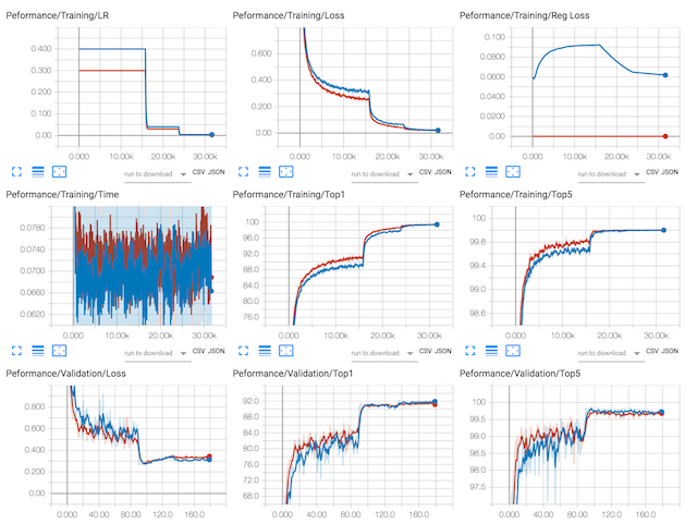
The diagram below shows the training of Resnet20/CIFAR10 using Group Lasso regularization on entire layers (in blue) vs. training Resnet20/CIFAR10 baseline (in red). You may notice several interesting things:
1. The LR-decay policy is the same, but the two sessions start with different initial LR values.
2. The data-loss of the regularized training follows the same shape as the un-regularized training (baseline), and eventually the two seem to merge.
3. We see similar behavior in the validation Top1 and Top5 accuracy results, but the regularized training eventually performs better.
4. In the top right corner we see the behavior of the regularization loss (Reg Loss), which actually increases for some time, until the data-loss has a sharp drop (after ~16K mini-batches), at which point the regularization loss also starts dropping.
This regularization yields 5 layers with zeroed weight tensors. We load this model, remove the 5 layers, and start the fine tuning of the weights. This process of layer removal is specific to ResNet for CIFAR, which we altered by adding code to skip over layers during the forward path. When you export to ONNX, the removed layers do not participate in the forward path, so they don't get incarnated.
We managed to remove 5 of the 16 3x3 convolution layers which dominate the computation time. It's not bad, but we probably could have done better.
Fine-tuning
During the fine-tuning process, because the removed layers do not participate in the forward path, they do not appear in the backward path and are not backpropogated: therefore they are completely disconnected from the network.
We copy the checkpoint file of the regularized model to checkpoint_trained_4D_regularized_5Lremoved.pth.tar.
Distiller schedule: distiller/examples/ssl/ssl_4D-removal_finetuning.yaml
$ time python3 compress_classifier.py --arch resnet20_cifar ../data.cifar10 -p=50 --lr=0.1 --epochs=250 --resume=../cifar10/resnet20/checkpoint_trained_4D_regularized_5Lremoved.pth.tar --compress=../ssl/ssl_4D-removal_finetuning.yaml -j=1 --deterministic
Results
Our baseline results for ResNet20 Cifar are: Top1=91.450 and Top5=99.750
We used Distiller's GroupLassoRegularizer to remove 5 layers from Resnet20 (CIFAR10) with no degradation of the accuracies.
The regularized model exhibits really poor classification abilities:
$ time python3 compress_classifier.py --arch resnet20_cifar  ../data.cifar10 -p=50 --resume=../cifar10/resnet20/checkpoint_trained_4D_regularized_5Lremoved.pth.tar --evaluate

=> loading checkpoint ../cifar10/resnet20/checkpoint_trained_4D_regularized_5Lremoved.pth.tar
   best top@1: 90.620
Loaded compression schedule from checkpoint (epoch 179)
Removing layer: module.layer1.0.conv1 [layer=0 block=0 conv=0]
Removing layer: module.layer1.0.conv2 [layer=0 block=0 conv=1]
Removing layer: module.layer1.1.conv1 [layer=0 block=1 conv=0]
Removing layer: module.layer1.1.conv2 [layer=0 block=1 conv=1]
Removing layer: module.layer2.2.conv2 [layer=1 block=2 conv=1]
Files already downloaded and verified
Files already downloaded and verified
Dataset sizes:
        training=45000
        validation=5000
        test=10000
--- test ---------------------
10000 samples (256 per mini-batch)
==> Top1: 22.290    Top5: 68.940    Loss: 5.172
However, after fine-tuning, we recovered most of the accuracies loss, but not quite all of it: Top1=91.020 and Top5=99.670
We didn't spend time trying to wrestle with this network, and therefore didn't achieve SSL's published results (which showed that they managed to remove 6 layers and at the same time increase accuracies).
Pruning Filters for Efficient ConvNets
Quoting the authors directly:
We present an acceleration method for CNNs, where we prune filters from CNNs that are identified as having a small effect on the output accuracy. By removing whole filters in the network together with their connecting feature maps, the computation costs are reduced significantly. In contrast to pruning weights, this approach does not result in sparse connectivity patterns. Hence, it does not need the support of sparse convolution libraries and can work with existing efficient BLAS libraries for dense matrix multiplications.
The implementation of the research by Hao et al. required us to add filter-pruning sensitivity analysis, and support for "network thinning".
After performing filter-pruning sensitivity analysis to assess which layers are more sensitive to the pruning of filters, we execute distiller.L1RankedStructureParameterPruner once in order to rank the filters of each layer by their L1-norm values, and then we prune the schedule-prescribed sparsity level.
- Distiller schedule:
distiller/examples/pruning_filters_for_efficient_convnets/resnet56_cifar_filter_rank.yaml
The excerpt from the schedule, displayed below, shows how we declare the L1RankedStructureParameterPruner. This class currently ranks filters only, but because in the future this class may support ranking of various structures, you need to specify for each parameter both the target sparsity level, and the structure type ('3D' is filter-wise pruning).
pruners:
  filter_pruner:
    class: 'L1RankedStructureParameterPruner'
    reg_regims:
      'module.layer1.0.conv1.weight': [0.6, '3D']
      'module.layer1.1.conv1.weight': [0.6, '3D']
      'module.layer1.2.conv1.weight': [0.6, '3D']
      'module.layer1.3.conv1.weight': [0.6, '3D']
In the policy, we specify that we want to invoke this pruner once, at epoch 180. Because we are starting from a network which was trained for 180 epochs (see Baseline training below), the filter ranking is performed right at the outset of this schedule.
policies:
  - pruner:
      instance_name: filter_pruner
    epochs: [180]
Following the pruning, we want to "physically" remove the pruned filters from the network, which involves reconfiguring the Convolutional layers and the parameter tensors. When we remove filters from Convolution layer n we need to perform several changes to the network:
1. Shrink layer n's weights tensor, leaving only the "important" filters.
2. Configure layer n's .out_channels member to its new, smaller, value.
3. If a BN layer follows layer n, then it also needs to be reconfigured and its scale and shift parameter vectors need to be shrunk.
4. If a Convolution layer follows the BN layer, then it will have less input channels which requires reconfiguration and shrinking of its weights.
All of this is performed by distiller.ResnetCifarFilterRemover which is also scheduled at epoch 180. We call this process "network thinning".
extensions:
  net_thinner:
      class: 'FilterRemover'
      thinning_func_str: remove_filters
      arch: 'resnet56_cifar'
      dataset: 'cifar10'
Network thinning requires us to understand the layer connectivity and data-dependency of the DNN, and we are working on a robust method to perform this. On networks with topologies similar to ResNet (residuals) and GoogLeNet (inception), which have several inputs and outputs to/from Convolution layers, there is extra details to consider.
Our current implementation is specific to certain layers in ResNet and is a bit fragile. We will continue to improve and generalize this.
Baseline training
We started by training the baseline ResNet56-Cifar dense network (180 epochs) since we didn't have a pre-trained model.
- Distiller schedule:
distiller/examples/pruning_filters_for_efficient_convnets/resnet56_cifar_baseline_training.yaml
Results
We trained a ResNet56-Cifar10 network and achieve accuracy results which are on-par with published results: Top1: 92.970 and Top5: 99.740.
We used Hao et al.'s algorithm to remove 37.3% of the original convolution MACs, while maintaining virtually the same accuracy as the baseline: Top1: 92.830 and Top5: 99.760