Using the sample application
The Distiller repository contains a sample application, distiller/examples/classifier_compression/compress_classifier.py, and a set of scheduling files which demonstrate Distiller's features. Following is a brief discussion of how to use this application and the accompanying schedules.
You might also want to refer to the following resources:
- An explanation of the scheduler file format.
- An in-depth discussion of how we used these schedule files to implement several state-of-the-art DNN compression research papers.
The sample application supports various features for compression of image classification DNNs, and gives an example of how to integrate distiller in your own application. The code is documented and should be considered the best source of documentation, but we provide some elaboration here.
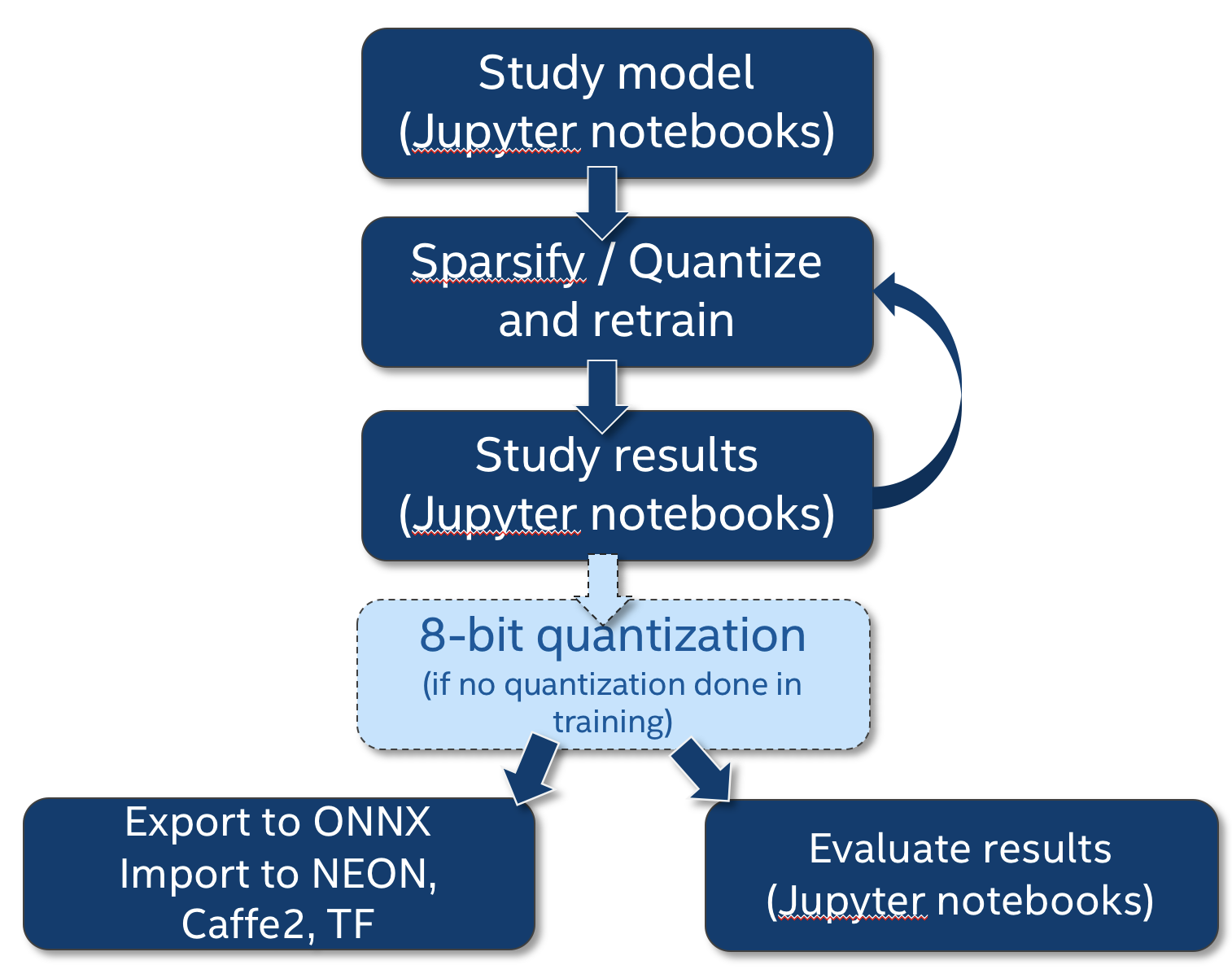
This diagram shows how where compress_classifier.py fits in the compression workflow, and how we integrate the Jupyter notebooks as part of our research work.
Command line arguments
To get help on the command line arguments, invoke:
$ python3 compress_classifier.py --help
For example:
$ time python3 compress_classifier.py -a alexnet --lr 0.005 -p 50 ../../../data.imagenet -j 44 --epochs 90 --pretrained --compress=../sensitivity-pruning/alexnet.schedule_sensitivity.yaml

Parameters:
 +----+---------------------------+------------------+---------------+----------------+------------+------------+----------+----------+----------+------------+---------+----------+------------+
 |    | Name                      | Shape            |   NNZ (dense) |   NNZ (sparse) |   Cols (%) |   Rows (%) |   Ch (%) |   2D (%) |   3D (%) |   Fine (%) |     Std |     Mean |   Abs-Mean |
 |----+---------------------------+------------------+---------------+----------------+------------+------------+----------+----------+----------+------------+---------+----------+------------|
 |  0 | features.module.0.weight  | (64, 3, 11, 11)  |         23232 |          13411 |    0.00000 |    0.00000 |  0.00000 |  0.00000 |  0.00000 |   42.27359 | 0.14391 | -0.00002 |    0.08805 |
 |  1 | features.module.3.weight  | (192, 64, 5, 5)  |        307200 |         115560 |    0.00000 |    0.00000 |  0.00000 |  1.91243 |  0.00000 |   62.38281 | 0.04703 | -0.00250 |    0.02289 |
 |  2 | features.module.6.weight  | (384, 192, 3, 3) |        663552 |         256565 |    0.00000 |    0.00000 |  0.00000 |  6.18490 |  0.00000 |   61.33445 | 0.03354 | -0.00184 |    0.01803 |
 |  3 | features.module.8.weight  | (256, 384, 3, 3) |        884736 |         315065 |    0.00000 |    0.00000 |  0.00000 |  6.96411 |  0.00000 |   64.38881 | 0.02646 | -0.00168 |    0.01422 |
 |  4 | features.module.10.weight | (256, 256, 3, 3) |        589824 |         186938 |    0.00000 |    0.00000 |  0.00000 | 15.49225 |  0.00000 |   68.30614 | 0.02714 | -0.00246 |    0.01409 |
 |  5 | classifier.1.weight       | (4096, 9216)     |      37748736 |        3398881 |    0.00000 |    0.21973 |  0.00000 |  0.21973 |  0.00000 |   90.99604 | 0.00589 | -0.00020 |    0.00168 |
 |  6 | classifier.4.weight       | (4096, 4096)     |      16777216 |        1782769 |    0.21973 |    3.46680 |  0.00000 |  3.46680 |  0.00000 |   89.37387 | 0.00849 | -0.00066 |    0.00263 |
 |  7 | classifier.6.weight       | (1000, 4096)     |       4096000 |         994738 |    3.36914 |    0.00000 |  0.00000 |  0.00000 |  0.00000 |   75.71440 | 0.01718 |  0.00030 |    0.00778 |
 |  8 | Total sparsity:           | -                |      61090496 |        7063928 |    0.00000 |    0.00000 |  0.00000 |  0.00000 |  0.00000 |   88.43694 | 0.00000 |  0.00000 |    0.00000 |
 +----+---------------------------+------------------+---------------+----------------+------------+------------+----------+----------+----------+------------+---------+----------+------------+
 2018-04-04 21:30:52,499 - Total sparsity: 88.44

 2018-04-04 21:30:52,499 - --- validate (epoch=89)-----------
 2018-04-04 21:30:52,499 - 128116 samples (256 per mini-batch)
 2018-04-04 21:31:04,646 - Epoch: [89][   50/  500]    Loss 2.175988    Top1 51.289063    Top5 74.023438
 2018-04-04 21:31:06,427 - Epoch: [89][  100/  500]    Loss 2.171564    Top1 51.175781    Top5 74.308594
 2018-04-04 21:31:11,432 - Epoch: [89][  150/  500]    Loss 2.159347    Top1 51.546875    Top5 74.473958
 2018-04-04 21:31:14,364 - Epoch: [89][  200/  500]    Loss 2.156857    Top1 51.585938    Top5 74.568359
 2018-04-04 21:31:18,381 - Epoch: [89][  250/  500]    Loss 2.152790    Top1 51.707813    Top5 74.681250
 2018-04-04 21:31:22,195 - Epoch: [89][  300/  500]    Loss 2.149962    Top1 51.791667    Top5 74.755208
 2018-04-04 21:31:25,508 - Epoch: [89][  350/  500]    Loss 2.150936    Top1 51.827009    Top5 74.767857
 2018-04-04 21:31:29,538 - Epoch: [89][  400/  500]    Loss 2.150853    Top1 51.781250    Top5 74.763672
 2018-04-04 21:31:32,842 - Epoch: [89][  450/  500]    Loss 2.150156    Top1 51.828125    Top5 74.821181
 2018-04-04 21:31:35,338 - Epoch: [89][  500/  500]    Loss 2.150417    Top1 51.833594    Top5 74.817187
 2018-04-04 21:31:35,357 - ==> Top1: 51.838    Top5: 74.817    Loss: 2.150

 2018-04-04 21:31:35,364 - Saving checkpoint
 2018-04-04 21:31:39,251 - --- test ---------------------
 2018-04-04 21:31:39,252 - 50000 samples (256 per mini-batch)
 2018-04-04 21:31:51,512 - Test: [   50/  195]    Loss 1.487607    Top1 63.273438    Top5 85.695312
 2018-04-04 21:31:55,015 - Test: [  100/  195]    Loss 1.638043    Top1 60.636719    Top5 83.664062
 2018-04-04 21:31:58,732 - Test: [  150/  195]    Loss 1.833214    Top1 57.619792    Top5 80.447917
 2018-04-04 21:32:01,274 - ==> Top1: 56.606    Top5: 79.446    Loss: 1.893
Let's look at the command line again:
$ time python3 compress_classifier.py -a alexnet --lr 0.005 -p 50 ../../../data.imagenet -j 44 --epochs 90 --pretrained --compress=../sensitivity-pruning/alexnet.schedule_sensitivity.yaml
In this example, we prune a TorchVision pre-trained AlexNet network, using the following configuration:
- Learning-rate of 0.005
- Print progress every 50 mini-batches.
- Use 44 worker threads to load data (make sure to use something suitable for your machine).
- Run for 90 epochs. Torchvision's pre-trained models did not store the epoch metadata, so pruning starts at epoch 0. When you train and prune your own networks, the last training epoch is saved as a metadata with the model. Therefore, when you load such models, the first epoch is not 0, but it is the last training epoch.
- The pruning schedule is provided in
alexnet.schedule_sensitivity.yaml - Log files are written to directory
logs.
Examples
Distiller comes with several example schedules which can be used together with compress_classifier.py.
These example schedules (YAML) files, contain the command line that is used in order to invoke the schedule (so that you can easily recreate the results in your environment), together with the results of the pruning or regularization. The results usually contain a table showing the sparsity of each of the model parameters, together with the validation and test top1, top5 and loss scores.
For more details on the example schedules, you can refer to the coverage of the Model Zoo.
- examples/agp-pruning:
- Automated Gradual Pruning (AGP) on MobileNet and ResNet18 (ImageNet dataset)
- Automated Gradual Pruning (AGP) on MobileNet and ResNet18 (ImageNet dataset)
- examples/hybrid:
- AlexNet AGP with 2D (kernel) regularization (ImageNet dataset)
- AlexNet sensitivity pruning with 2D regularization
- examples/network_slimming:
- ResNet20 Network Slimming (this is work-in-progress)
- ResNet20 Network Slimming (this is work-in-progress)
- examples/pruning_filters_for_efficient_convnets:
- ResNet56 baseline training (CIFAR10 dataset)
- ResNet56 filter removal using filter ranking
- examples/sensitivity_analysis:
- Element-wise pruning sensitivity-analysis:
- AlexNet (ImageNet)
- MobileNet (ImageNet)
- ResNet18 (ImageNet)
- ResNet20 (CIFAR10)
- ResNet34 (ImageNet)
- Filter-wise pruning sensitivity-analysis:
- ResNet20 (CIFAR10)
- ResNet56 (CIFAR10)
- examples/sensitivity-pruning:
- AlexNet sensitivity pruning with Iterative Pruning
- AlexNet sensitivity pruning with One-Shot Pruning
- examples/ssl:
- ResNet20 baseline training (CIFAR10 dataset)
- Structured Sparsity Learning (SSL) with layer removal on ResNet20
- SSL with channels removal on ResNet20
- examples/quantization:
- AlexNet w. Batch-Norm (base FP32 + DoReFa)
- Pre-activation ResNet20 on CIFAR10 (base FP32 + DoReFa)
- Pre-activation ResNet18 on ImageNEt (base FP32 + DoReFa)
Experiment reproducibility
Experiment reproducibility is sometimes important. Pete Warden recently expounded about this in his blog.
PyTorch's support for deterministic execution requires us to use only one thread for loading data (other wise the multi-threaded execution of the data loaders can create random order and change the results), and to set the seed of the CPU and GPU PRNGs. Using the --deterministic command-line flag and setting j=1 will produce reproducible results (for the same PyTorch version).
Performing pruning sensitivity analysis
Distiller supports element-wise and filter-wise pruning sensitivity analysis. In both cases, L1-norm is used to rank which elements or filters to prune. For example, when running filter-pruning sensitivity analysis, the L1-norm of the filters of each layer's weights tensor are calculated, and the bottom x% are set to zero.
The analysis process is quite long, because currently we use the entire test dataset to assess the accuracy performance at each pruning level of each weights tensor. Using a small dataset for this would save much time and we plan on assessing if this will provide sufficient results.
Results are output as a CSV file (sensitivity.csv) and PNG file (sensitivity.png). The implementation is in distiller/sensitivity.py and it contains further details about process and the format of the CSV file.
The example below performs element-wise pruning sensitivity analysis on ResNet20 for CIFAR10:
$ python3 compress_classifier.py -a resnet20_cifar ../../../data.cifar10/ -j=1 --resume=../cifar10/resnet20/checkpoint_trained_dense.pth.tar --sense=element
The sense command-line argument can be set to either element or filter, depending on the type of analysis you want done.
There is also a Jupyter notebook with example invocations, outputs and explanations.
Post-Training Quantization
The following example qunatizes ResNet18 for ImageNet:
$ python3 compress_classifier.py -a resnet18 ../../../data.imagenet --pretrained --quantize-eval --evaluate
See here for more details on how to invoke post-training quantization from the command line.
A checkpoint with the quantized model will be dumped in the run directory. It will contain the quantized model parameters (the data type will still be FP32, but the values will be integers). The calculated quantization parameters (scale and zero-point) are stored as well in each quantized layer.
For more examples of post-training quantization see here.
Summaries
You can use the sample compression application to generate model summary reports, such as the attributes and compute summary report (see screen capture below). You can log sparsity statistics (written to console and CSV file), performance, optimizer and model information, and also create a PNG image of the DNN. Creating a PNG image is an experimental feature (it relies on features which are not available on PyTorch 3.1 and that we hope will be available in PyTorch's next release), so to use it you will need to compile the PyTorch master branch, and hope for the best ;-).
$ python3 compress_classifier.py --resume=../ssl/checkpoints/checkpoint_trained_ch_regularized_dense.pth.tar -a=resnet20_cifar ../../../data.cifar10 --summary=compute
Generates:
+----+------------------------------+--------+----------+-----------------+--------------+-----------------+--------------+------------------+---------+
|    | Name                         | Type   | Attrs    | IFM             |   IFM volume | OFM             |   OFM volume |   Weights volume |    MACs |
|----+------------------------------+--------+----------+-----------------+--------------+-----------------+--------------+------------------+---------|
|  0 | module.conv1                 | Conv2d | k=(3, 3) | (1, 3, 32, 32)  |         3072 | (1, 16, 32, 32) |        16384 |              432 |  442368 |
|  1 | module.layer1.0.conv1        | Conv2d | k=(3, 3) | (1, 16, 32, 32) |        16384 | (1, 16, 32, 32) |        16384 |             2304 | 2359296 |
|  2 | module.layer1.0.conv2        | Conv2d | k=(3, 3) | (1, 16, 32, 32) |        16384 | (1, 16, 32, 32) |        16384 |             2304 | 2359296 |
|  3 | module.layer1.1.conv1        | Conv2d | k=(3, 3) | (1, 16, 32, 32) |        16384 | (1, 16, 32, 32) |        16384 |             2304 | 2359296 |
|  4 | module.layer1.1.conv2        | Conv2d | k=(3, 3) | (1, 16, 32, 32) |        16384 | (1, 16, 32, 32) |        16384 |             2304 | 2359296 |
|  5 | module.layer1.2.conv1        | Conv2d | k=(3, 3) | (1, 16, 32, 32) |        16384 | (1, 16, 32, 32) |        16384 |             2304 | 2359296 |
|  6 | module.layer1.2.conv2        | Conv2d | k=(3, 3) | (1, 16, 32, 32) |        16384 | (1, 16, 32, 32) |        16384 |             2304 | 2359296 |
|  7 | module.layer2.0.conv1        | Conv2d | k=(3, 3) | (1, 16, 32, 32) |        16384 | (1, 32, 16, 16) |         8192 |             4608 | 1179648 |
|  8 | module.layer2.0.conv2        | Conv2d | k=(3, 3) | (1, 32, 16, 16) |         8192 | (1, 32, 16, 16) |         8192 |             9216 | 2359296 |
|  9 | module.layer2.0.downsample.0 | Conv2d | k=(1, 1) | (1, 16, 32, 32) |        16384 | (1, 32, 16, 16) |         8192 |              512 |  131072 |
| 10 | module.layer2.1.conv1        | Conv2d | k=(3, 3) | (1, 32, 16, 16) |         8192 | (1, 32, 16, 16) |         8192 |             9216 | 2359296 |
| 11 | module.layer2.1.conv2        | Conv2d | k=(3, 3) | (1, 32, 16, 16) |         8192 | (1, 32, 16, 16) |         8192 |             9216 | 2359296 |
| 12 | module.layer2.2.conv1        | Conv2d | k=(3, 3) | (1, 32, 16, 16) |         8192 | (1, 32, 16, 16) |         8192 |             9216 | 2359296 |
| 13 | module.layer2.2.conv2        | Conv2d | k=(3, 3) | (1, 32, 16, 16) |         8192 | (1, 32, 16, 16) |         8192 |             9216 | 2359296 |
| 14 | module.layer3.0.conv1        | Conv2d | k=(3, 3) | (1, 32, 16, 16) |         8192 | (1, 64, 8, 8)   |         4096 |            18432 | 1179648 |
| 15 | module.layer3.0.conv2        | Conv2d | k=(3, 3) | (1, 64, 8, 8)   |         4096 | (1, 64, 8, 8)   |         4096 |            36864 | 2359296 |
| 16 | module.layer3.0.downsample.0 | Conv2d | k=(1, 1) | (1, 32, 16, 16) |         8192 | (1, 64, 8, 8)   |         4096 |             2048 |  131072 |
| 17 | module.layer3.1.conv1        | Conv2d | k=(3, 3) | (1, 64, 8, 8)   |         4096 | (1, 64, 8, 8)   |         4096 |            36864 | 2359296 |
| 18 | module.layer3.1.conv2        | Conv2d | k=(3, 3) | (1, 64, 8, 8)   |         4096 | (1, 64, 8, 8)   |         4096 |            36864 | 2359296 |
| 19 | module.layer3.2.conv1        | Conv2d | k=(3, 3) | (1, 64, 8, 8)   |         4096 | (1, 64, 8, 8)   |         4096 |            36864 | 2359296 |
| 20 | module.layer3.2.conv2        | Conv2d | k=(3, 3) | (1, 64, 8, 8)   |         4096 | (1, 64, 8, 8)   |         4096 |            36864 | 2359296 |
| 21 | module.fc                    | Linear |          | (1, 64)         |           64 | (1, 10)         |           10 |              640 |     640 |
+----+------------------------------+--------+----------+-----------------+--------------+-----------------+--------------+------------------+---------+
Total MACs: 40,813,184
Using TensorBoard
Google's TensorBoard is an excellent tool for visualizing the progress of DNN training. Distiller's logger supports writing performance indicators and parameter statistics in a file format that can be read by TensorBoard.
To view the graphs, invoke the TensorBoard server. For example:
$ tensorboard --logdir=logs
Collecting activations statistics
In CNNs with ReLU layers, ReLU activations (feature-maps) also exhibit a nice level of sparsity (50-60% sparsity is typical).
You can collect activation statistics using the --act_stats command-line flag.
For example:
$ python3 compress_classifier.py -a=resnet56_cifar -p=50 ../../../data.cifar10 --resume=checkpoint.resnet56_cifar_baseline.pth.tar --act-stats=test -e
The test parameter indicates that, in this example, we want to collect activation statistics during the test phase. Note that we also used the -e command-line argument to indicate that we want to run a test phase. The other two legal parameter values are train and valid which collect activation statistics during the training and validation phases, respectively.
Collectors and their collaterals
An instance of a subclass of ActivationStatsCollector can be used to collect activation statistics. Currently, ActivationStatsCollector has two types of subclasses: SummaryActivationStatsCollector and RecordsActivationStatsCollector.
Instances of SummaryActivationStatsCollector compute the mean of some statistic of the activation. It is rather
light-weight and quicker than collecting a record per activation. The statistic function is configured in the constructor.
In the sample compression application, compress_classifier.py, we create a dictionary of collectors. For example:
SummaryActivationStatsCollector(model,
                                "sparsity",
                                lambda t: 100 * distiller.utils.sparsity(t))
The lambda expression is invoked per activation encountered during forward passes, and the value it returns (in this case, the sparsity of the activation tensors, multiplied by 100) is stored in module.sparsity ("sparsity" is this collector's name). To access the statistics, you can invoke collector.value(), or you can access each module's data directly.
Another type of collector is RecordsActivationStatsCollector which computes a hard-coded set of activations statistics and collects a
record per activation. For obvious reasons, this is slower than instances of SummaryActivationStatsCollector.ActivationStatsCollector default to collecting activations statistics only on the output activations of ReLU layers, but we can choose any layer type we want. In the example below we collect statistics from outputs of torch.nn.Conv2d layers.
RecordsActivationStatsCollector(model, classes=[torch.nn.Conv2d])
Collectors can write their data to Excel workbooks (which are named using the collector's name), by invoking collector.to_xlsx(path_to_workbook). In compress_classifier.py we currently create four different collectors which you can selectively disable. You can also add other statistics collectors and use a different function to compute your new statistic.
collectors = missingdict({
    "sparsity":      SummaryActivationStatsCollector(model, "sparsity",
                                                     lambda t: 100 * distiller.utils.sparsity(t)),
    "l1_channels":   SummaryActivationStatsCollector(model, "l1_channels",
                                                     distiller.utils.activation_channels_l1),
    "apoz_channels": SummaryActivationStatsCollector(model, "apoz_channels",
                                                     distiller.utils.activation_channels_apoz),
    "records":       RecordsActivationStatsCollector(model, classes=[torch.nn.Conv2d])})
By default, these Collectors write their data to files in the active log directory.
You can use a utility function, distiller.log_activation_statsitics, to log the data of an ActivationStatsCollector instance to one of the backend-loggers. For an example, the code below logs the "sparsity" collector to a TensorBoard log file.
distiller.log_activation_statsitics(epoch, "train", loggers=[tflogger],
                                    collector=collectors["sparsity"])
Caveats
Distiller collects activations statistics using PyTorch's forward-hooks mechanism. Collectors iteratively register the modules' forward-hooks, and collectors are called during the forward traversal and get exposed to activation data. Registering for forward callbacks is performed like this:
module.register_forward_hook
This makes apparent two limitations of this mechanism:
- We can only register on PyTorch modules. This means that we can't register on the forward hook of a functionals such as
torch.nn.functional.reluandtorch.nn.functional.max_pool2d.
Therefore, you may need to replace functionals with their module alternative. For example:
class MadeUpNet(nn.Module):
    def __init__(self):
        super().__init__()
        self.conv1 = nn.Conv2d(3, 6, 5)

    def forward(self, x):
        x = F.relu(self.conv1(x))
        return x
Can be changed to:
class MadeUpNet(nn.Module):
    def __init__(self):
        super().__init__()
        self.conv1 = nn.Conv2d(3, 6, 5)
        self.relu = nn.ReLU(inplace=True)

    def forward(self, x):
        x = self.relu(self.conv1(x))
        return x
- We can only use a module instance once in our models. If we use the same module several times, then we can't determine which node in the graph has invoked the callback, because the PyTorch callback signature
def hook(module, input, output)doesn't provide enough contextual information.
TorchVision's ResNet is an example of a model that uses the same instance of nn.ReLU multiple times:
class BasicBlock(nn.Module):
    expansion = 1
    def __init__(self, inplanes, planes, stride=1, downsample=None):
        super(BasicBlock, self).__init__()
        self.conv1 = conv3x3(inplanes, planes, stride)
        self.bn1 = nn.BatchNorm2d(planes)
        self.relu = nn.ReLU(inplace=True)
        self.conv2 = conv3x3(planes, planes)
        self.bn2 = nn.BatchNorm2d(planes)
        self.downsample = downsample
        self.stride = stride

    def forward(self, x):
        residual = x
        out = self.conv1(x)
        out = self.bn1(out)
        out = self.relu(out)                    # <================
        out = self.conv2(out)
        out = self.bn2(out)
        if self.downsample is not None:
            residual = self.downsample(x)
        out += residual
        out = self.relu(out)                    # <================
        return out
In Distiller we changed ResNet to use multiple instances of nn.ReLU, and each instance is used only once:
class BasicBlock(nn.Module):
    expansion = 1
    def __init__(self, inplanes, planes, stride=1, downsample=None):
        super(BasicBlock, self).__init__()
        self.conv1 = conv3x3(inplanes, planes, stride)
        self.bn1 = nn.BatchNorm2d(planes)
        self.relu1 = nn.ReLU(inplace=True)
        self.conv2 = conv3x3(planes, planes)
        self.bn2 = nn.BatchNorm2d(planes)
        self.relu2 = nn.ReLU(inplace=True)
        self.downsample = downsample
        self.stride = stride

    def forward(self, x):
        residual = x
        out = self.conv1(x)
        out = self.bn1(out)
        out = self.relu1(out)                   # <================
        out = self.conv2(out)
        out = self.bn2(out)
        if self.downsample is not None:
            residual = self.downsample(x)
        out += residual
        out = self.relu2(out)                   # <================
        return out
Using the Jupyter notebooks
The Jupyter notebooks contain many examples of how to use the statistics summaries generated by Distiller. They are explained in a separate page.
Generating this documentation
Install mkdocs and the required packages by executing:
$ pip3 install -r doc-requirements.txt
To build the project documentation run:
$ cd distiller/docs-src
$ mkdocs build --clean
This will create a folder named 'site' which contains the documentation website. Open distiller/docs/site/index.html to view the documentation home page.